Typical shot selection: From Zion’s floater to Dame’s logo shot
Rui Qiu
Updated on 2021-10-19.
It’s a pity that the shot attempt data from chapter 3 hasn’t been utilized since then. Luckily, this won’t be the case anymore. This chapter aims to perform associate rule mining (ARM) on a portion of NBA shot data. An explanation will be given later on why only partial data is used here.
The ARM will identify a list of controlled frequent
itemsets, thus leading to a list of controlled frequent
rules. They are controlled because only rules contain the information of if this specific shot is
made matter. Otherwise, rules such as {shottype=Arc3=>value=3} will be
valid for sure but not informative.
Although the shot data won’t provide any highlights of a player’s signature move, it will hopefully give some insights into his favorite shot selection. To some extent, this also draws the boundary of a player’s hot zone.
Setup
Script: arm-shots.R
Intermediate transaction rules data:
Intermediate frequent itemsets and rules:
Output JSON: network-data.json
The script above fulfills all the tasks in this chapter, including both ARM and network visualization.
The packages used in the script are:
{tidyverse}for standard data analytics pipelines{arules}for associate rule mining{arulesViz},{networkD3}and{visNetwork}for network visualization
Data cleaning
The data cleaning procedure starts by loading a previously cleaned, tidy data set. Since the ARM has a specific requirement for categorical variables as the input, variables will be factorized accordingly.
In short, we are doing the following three types of data mutation:
- Transform numeric data to factors
- Transform logical data to factors with details
- Transform NA to data as well.
Unsurprisingly, since the data preserved lots of NAs in some variables for the integrity of the data, it is relatively reasonable to discard them in this task. Are they providing some information? Yes. But are they providing enough information to be included in the rule? Not really. A trial run with NAs gives out many rules with uninterpretable items. Therefore, the following variables are considered to be the participants of rules:
player: the name of the shot taker.period: the time period of a game that the shot takes place.shottype: the specific type of the shot, e.g.,Arc3,Corner3, etc.value: either 2 pts or 3 pts.and1: whether the shot is fouled, and a free throw is given.made: whether the shot is made and corresponding pts are rewarded.
Associate rule mining
After that, the data frame will again be processed by the generic R function
as(), which coerces an object to another class, to transaction data. It can be
examined by inspect().
The transactions data is a single R object, therefore stored as an RDS file in the repository.
In addition, another copy of CSV is stored in the repository. And it can be viewed as an embedded Airtable spreadsheet. Due to this web design’s effective width limitation, screenshots won’t be an appropriate option to display the transaction dataset.
Apriori algorithm is an easy-to-implement and interpretable algorithm frequently used in ARM. It prunes all the combinations of itemsets by setting a few parameters.
The parameters used for the generation of these rules are:
support = 0.0001confidence = 0.5minlen = 6- And the RHS of the rule must be either
made=is_madeormade=not_made
These parameters generate hundreds of meaningful rules, which are listed in that embedded spreadsheet.
As mentioned above, although the complete set of rules should be more than what is presented here, many of them are meaningless, considering the goal of analyzing this dataset is to outline players’ typical shot selection. Therefore, the parameters are set to be:
The frequent itemsets and top rules listed below are stored as intermediate CSV files, also accessible in the repository. At the same, they are uploaded to an Airtable spreadsheet as well. You can observe different sets of data by switching the tabs.
Note: you can click on the burger menu button on top-left corner to switch tables.
Top itemsets
First, let’s take a look at some frequent items in all transactions.
Apparently, many star players’ signature shots are successfully retrieved. For instance:
- Stephen Curry’s tons of 3-pointer from the arc, both made and missed.
- Damian Lillard’s iconic logo shot.
-
Zion Williamson’s unguardable attack-the-rim (and possibly with and-1)
Top rules
Then, the rules are sorted by three metrics separately. For each metric, the top 15 results will be listed. You can switch the tabs of the spreadsheet above to view the datasets.
- Rank by support. This generally copies the results of the most frequent itemsets since support indicates how frequently the items appear in the dataset.
- Rank by confidence. This shows how often the rule has been found to be true. Compared to the top 15 rules by support, there are some differences.
- Rank by lift. The lift greater than 1 indicates that the two events (LHS and RHS) are dependent on one another. It shows that some players’ shot selections are frequent, but they are their major attacking approaches. And again, more signature shot selections are identified. All of the 15 typical shot selection combinations are 2-pointers. The top three are Zion and Giannis’ shots with and-1. How unstoppable!
More rules
Before jumping into the network visualization, let’s take a look at the shot rules dataset again. Suppose the LHS is filtered to be a particular player. In that case, a list of rules involving this player can be returned easily.
Again, the length of the output is controlled by the parameter. For example, by changing the
minlen to 2:
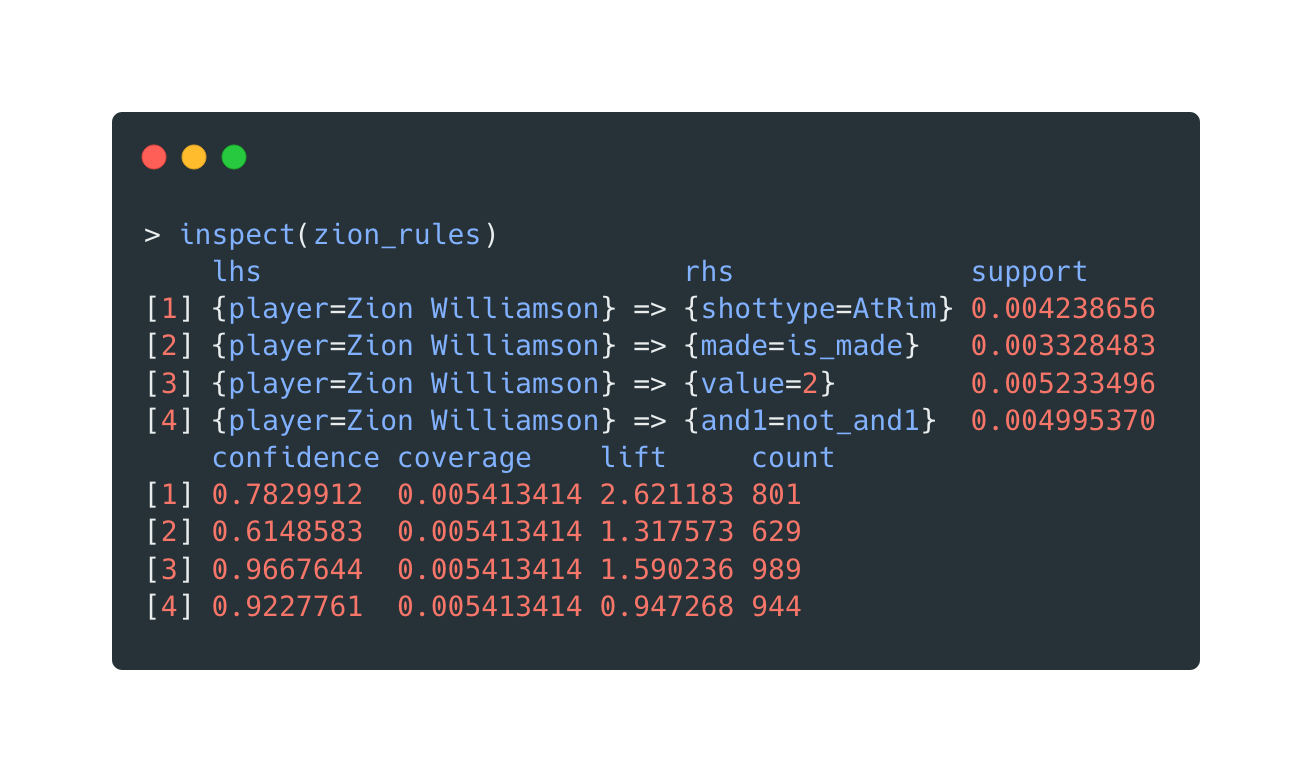
Open in new tab to see in full size.
Conclusion
To conclude, ARM is a basic rule-based machine learning method used to identify interesting relations between variables in a rather large dataset. The threshold used to define what a “strong” rule is, however, can be tuned by manual selection. Based on this method, a list of meaningful rules about NBA players and their shot selections are generated.
Network Viz
The network visualization is a perfect choice to demonstrate the interconnection among different rules and rules’ items. Too many rules can, of course, be visualized within one html widget, but it won’t be easy to be interact with. For the following three visualization packages, each only visualizes a partition of the rules data for the apparent aesthetic reason.
{arulesViz}
Two versions of networks are generated by the {arulesViz} package. They
are
essentially the same.
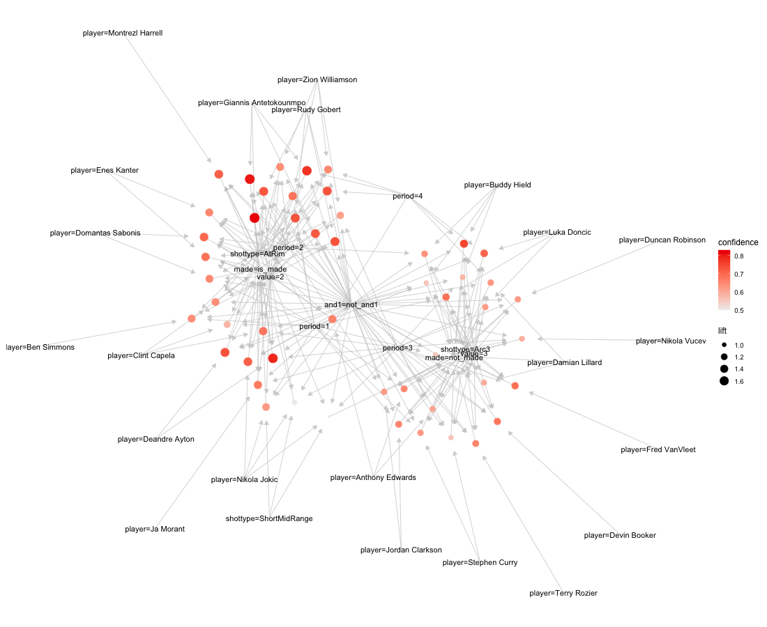
{arulesViz}.Open in new tab to see in full size.
Although the rules are ranked by support, the visual
cues focus
on the other two metrics. The associate rules are marked as red circles in the network. The darker
the
circle, the higher confidence it indicates. The larger,
the
higher lift it has. The ones in the corner, for example,
are the
rules of Zion Williamson and Giannis Antetokounmpos’ shot at the rim. There are also some nodes with
high
degrees, which means they are pretty common in many
rules. The
nodes with made=is_made and made=not_made are
automatically two with high traffic since any rule connects with either of them. Some other nodes,
which are
the variables used to describe a shot, are also connected by a large number of edges.
Data preparation
With the rule dataset and some basic knowledge of graph theory, we can transform the dataset into something more D3-friendly. Roughly speaking, the new datasets should contain nodes and edges, including some miscellaneous aspects like the group and the color of those elements.
Unlike the sub-dataset used by {arulesViz}, the one visualized by the
following two
packages uses the complete ruleset. Then we extract two subsets from the data,
- one containing top 50 made shots scenario in the 4th quarter ranked by counts,
- one containing only Zion Williamson and Giannis Antetokounmpos’ shot attempts.
The detailed data pipeline scripts are included in the R script under “Network Viz - data preparation.”
{networkD3}
Since {networkD3} utilizes D3.js, the index of records in
nodes and edges needs to subtract 1.
The network visualized above shows some common shot selections in the 4th quarter of an NBA game,
a.k.a,
“the clutch time.” The orange nodes are the associate rules, while the blue ones are shot variables
(including the player). The most common two variables are automatically
made=is_made and period=4, since all rules are
apparently
about these two. Then there are shottype=AtRim and
shottype=ShortMidRange. This might be explained by many tactics built on “safe
plays.”
Another cause might be filtering by counts, such that many risky but successful 3-pointer made are
excluded
due to small quantity.
To give some specific examples, the network features more plays like this:
And fewer like this:
{VisNetwork}
Even if they are not Giannis’ top choices,
Arc3,ShortMidrange, and
LongMidrange are in his arsenal. On the contrary, Zion is insanely efficient
with
AtRim (majorly because of his floaters and dunks).
The two clips below are examples of their typical shot attempts.
Zion's dunk:
Giannis' midrange, though relatively rare in previous seasons:
Sankey diagram
Last but not least, it just takes a one-liner to generate a Sankey diagram of a subset of rules by
networkD3::sankeyNetwork().
Although the diagram presents the same dataset as {VisNetwork} did, it
actually
unwraps in a more tidy manner. One can clearly tell the quantitative difference in each node by
grouping the
same variable with the same color.
Summary
In summary, the data scraped and cleaned from the last few weeks are finally put into action. By using ARM, one can quickly unearth the typical shot selection patterns among NBA players. With some proper data manipulation, even more, information is revealed with the assistance of network visualization.
For the development of modern basketball, splitting the data season by season will clearly highlight the changes in shot selections of a player, a team, or the whole league, which is an indicator of tactical changes. More importantly, ARM and networks can be utilized when dealing with tons of data. Imagine a scenario that an analyst needs to study the shot preferences of an opponent team. Therefore, they can extract the frequent rules in a flash instead of watching hundreds of hours of videotapes.
Admittedly, the dataset used in this chapter is barely a fraction of the entire shot scenario, as lots of other descriptive variables are removed for various reasons. If more data is provided, it’s definitely possible to build a more captivating list of basketball “rules” so that both analysts and ordinary audiences can read the game from another angle. Furthermore, a predictive model based on associate rule mining is practical to predict how threatening a shot could be. Thus, it could serve as one piece of the xT model we initially aim to build from the beginning.