A tale of two classifiers part 1

Mixed record data with R

Data and scripts

• Data: team-shots-TOR.csv

• Script: nb-svm-script.R

The data consists of Toronto Raptors’ shot attempt data (mostly from 2020-2021 season) with the following general structure (with both numeric and categorical features):

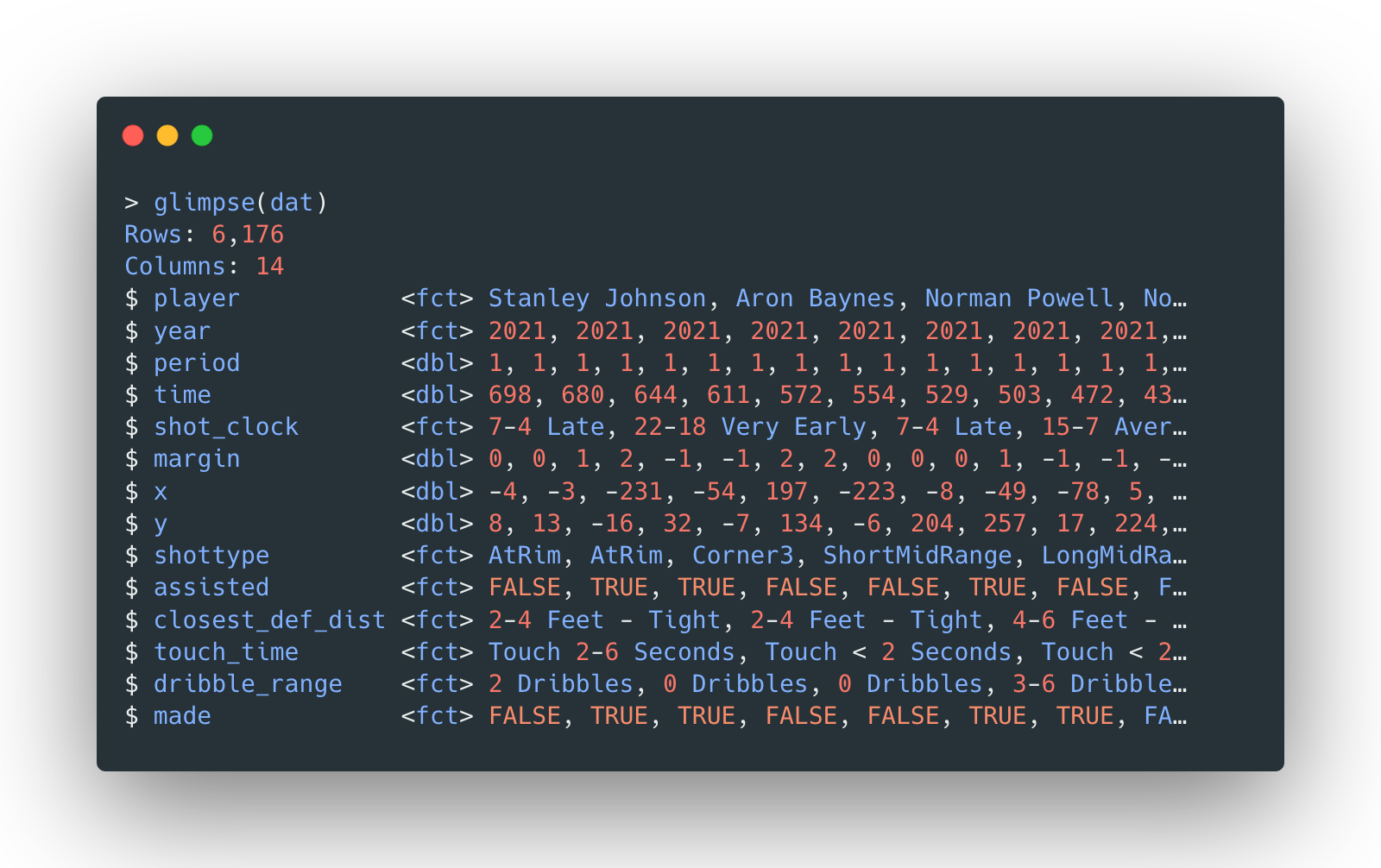
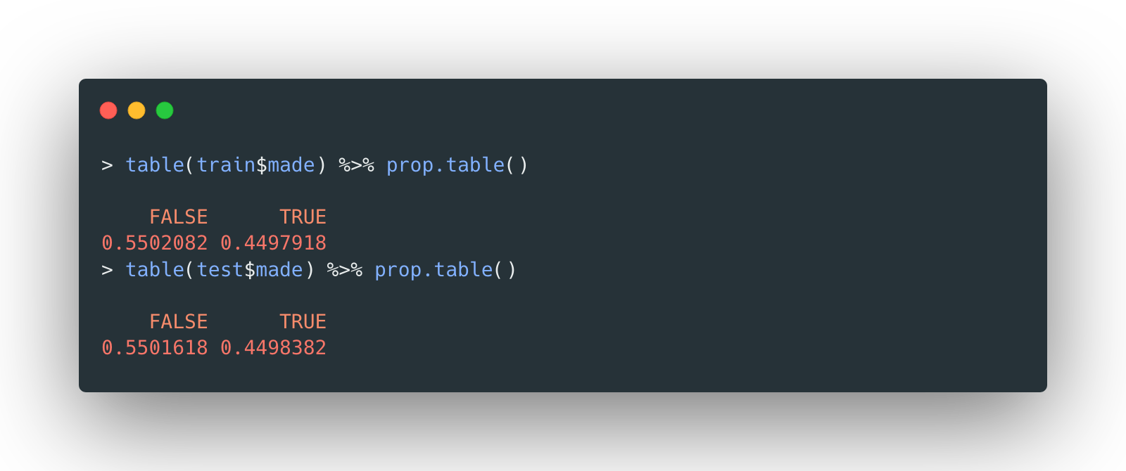
The data set is also split into a 70-30 train-test split, stratified by the result made.

Model tuning

{caret} package is used to conduct a 10-fold cross validation.

One naïve version of naïve bayes classifiers, without any parameter tuning, is concluded as below:

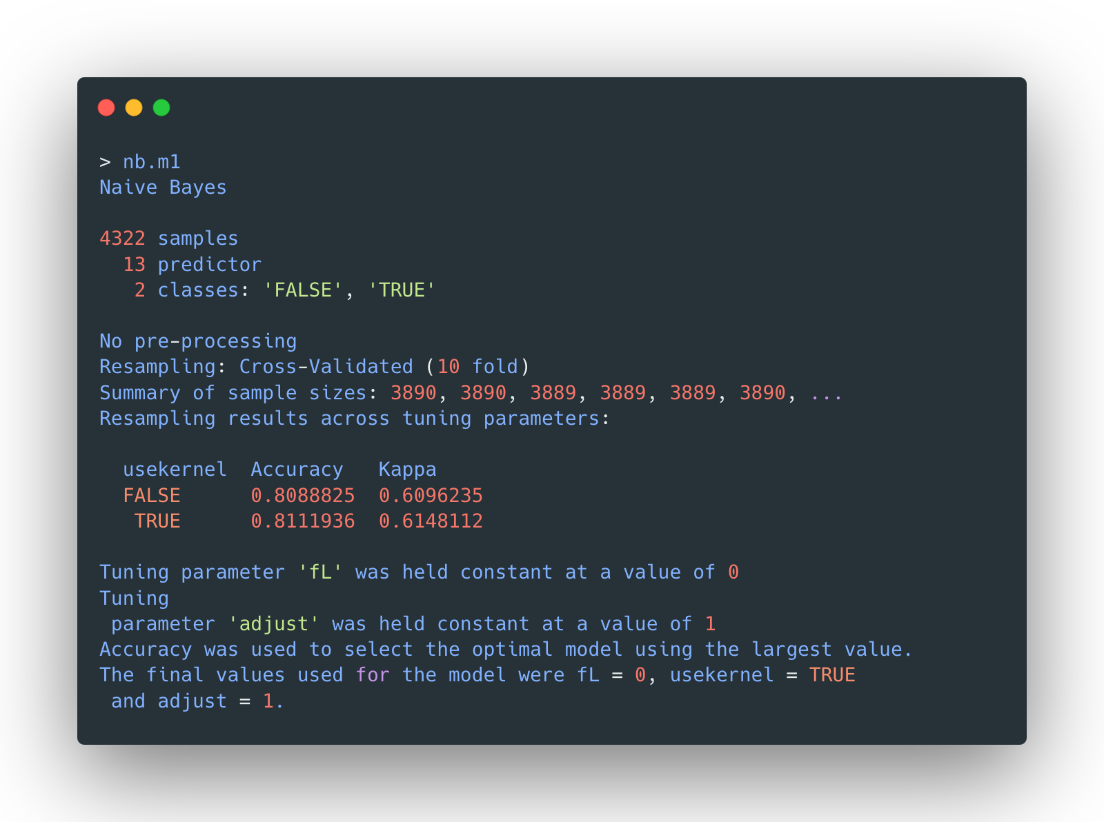
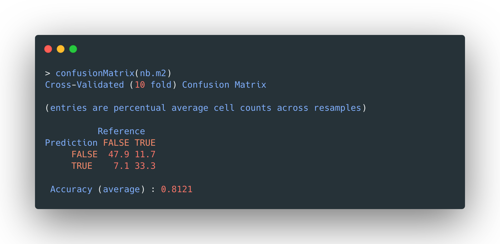
Take a look at its confusion matrix and mean accuracy:

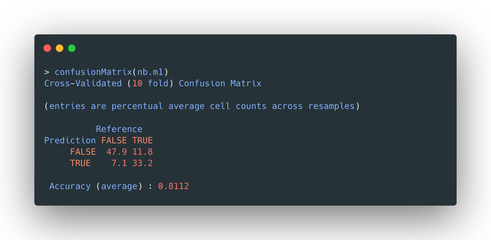
The overall accuracy is 81.12%, not bad. But apparently, the beauty of model selection is to fine tune some hyperparameters so that a model could improve itself.

The following three hyperparameters are involved:

• usekernel: use a kernel density estimate for continuous variables vs a Gaussian density estimate.
• adjust: adjust the bandwidth of the kernel density (larger numbers mean more flexible density estimate)
• fL: Laplace smoother

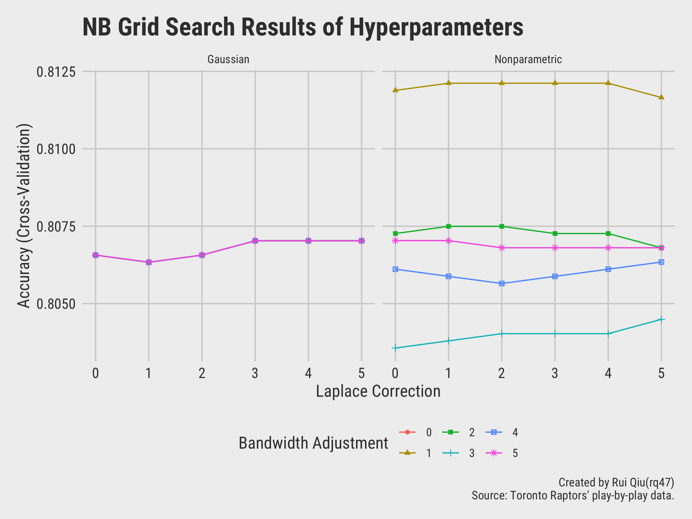
Again, the grid search approach is used to accomplish this mission. In addition, the numeric predictors are preprocessed with “center" and “scale”, i.e., standardization.

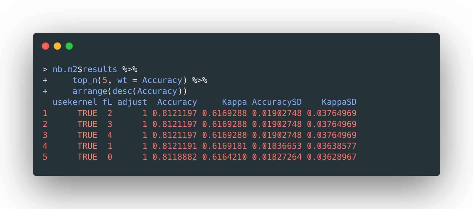
The resulted models are ordered by accuracy as the selection criterion. Top 5 of them are displayed below:

As the tuning process, it can be visualized as the following two charts as well:

The overall accuracy of tuned version naïve Bayes is 81.21%, slightly better than the untuned version.

Then the testing data is validated on selected naïve Bayes model, which returns the following confusion matrix:

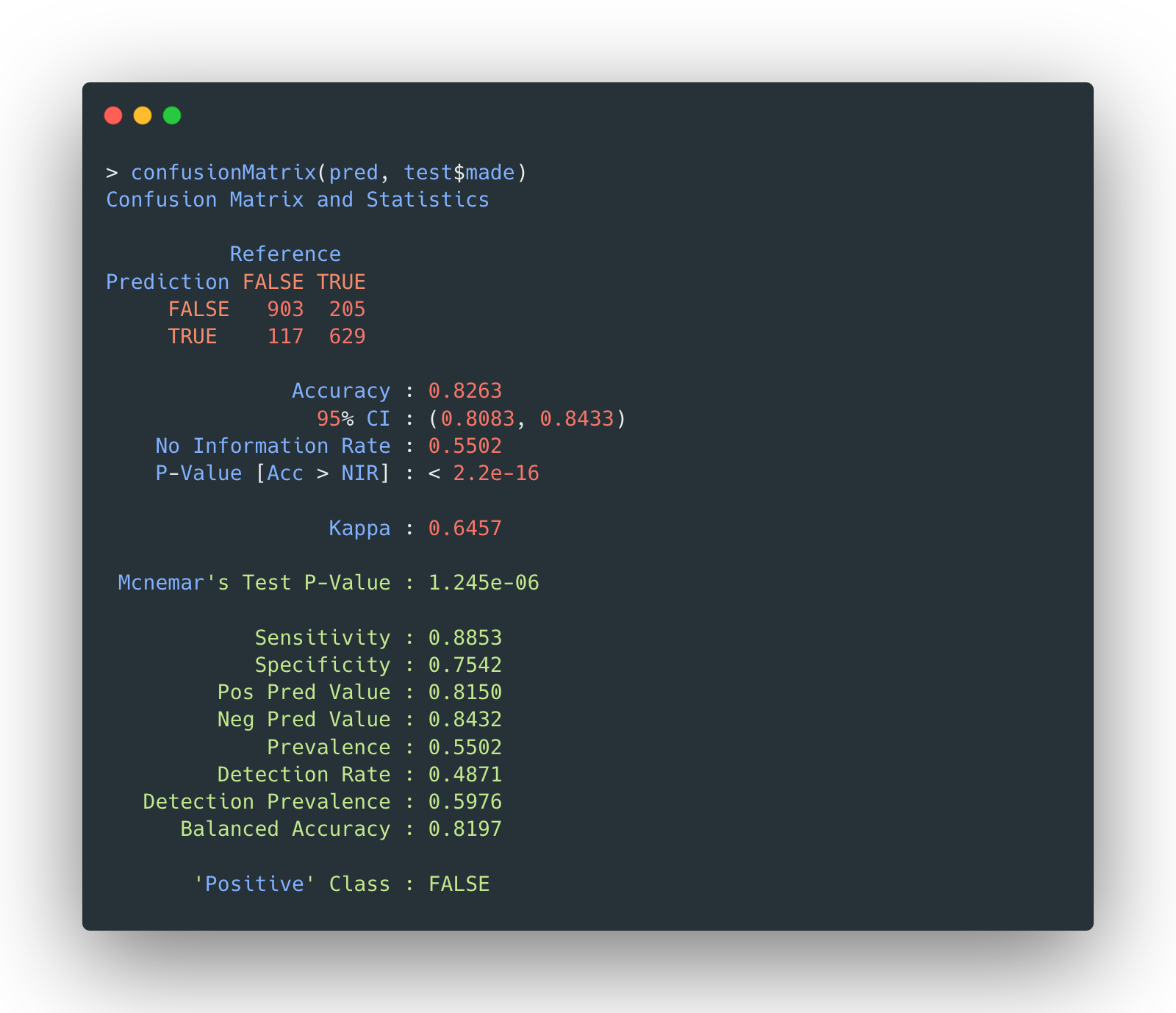
The result is very uplifting as the model actually outperforms itself with training data, which eventually reaches an accuracy of 82.63%.

Feature importance

The feature importance in an object of train is rather hard to extract when the naïve Bayes model is filled with imbalanced categorical data. Given the fact that some features include more than a dozen of possible categories, for example, the player has almost every active player on Toronto Raptors roaster from last season, therefore, an alternative approach to represent how relatively important those features are is to display all the conditional probabilities. The features which vary a lot between two possible target variables are the ones of greater importance.

Visualization of NB prediction

To see how the model works in practice, two visualizations are plotted to see the actual shots made/missed and the predicted shots made/missed.

It turns out most of the deviations between the reality and the prediction are in midranges and 45-degree three-pointers.

Finally, a visualization is carried out to show the overall prediction accuracy of a fine-tuned naïve Bayes classifier:

Interpretation

Recall previous attempts to predict if a shot is made with tree-based classifiers, the overall accuracy is barely over 50%. As mentioned last time, if a classifier, especially a binary classifier, only performs like flipping a coin, then it is really bad model.

Is it due to the nature of the data? The answer is, “it’s possible”from last time.

However, a very similar subset of data is used to capture the shot attempt pattern with a naïve Bayes classifier. The core idea is the following multinomial formula by Bayes theorem:

$p(\mathbf{x}|C_k)=\frac{(\sum^n_{i=1}x_i)!}{\prod^n_{i=1}x_i!}\prod^n_{i=1}p_{ki}^{x_i}$

where x’s are possible values of all the predictors.

Then the class C is selected by the argmax of such a product. It’s more or less like a voting procedure, the class results in a higher probability will be the predicted class of this record.

Intuitively, given a set of predictors, the classifier calculates the separate probabilities that could happen under a class C_k. Then the posterior probability is the joint probability of these separate independent probabilities.

However, one should note that in reality, the assumption of independence among features/variables is very rare.

Still, the naïve Bayes classifier gives a decent prediction to start this “tale of two classifiers.” More to be discussed in the next part of this portfolio.

Text data with Python

Data and scripts

• Data

  • Raw data
  • Cleaned data

• Script: reddit-nb-svm.ipynb

Just like the record data, the text data in this section is also from the tree-based classification chapter.

The data is preprocessed by removing stopwords, conversion to lower case, and then calculated as Tf-idf. What is different from last time is that the texts are not stripped as bigrams but unigrams this time.

Additionally, the target variable upvote_ratio is replaced by popularity, a categorical variable indicating how popular the thread is within the time span of a year. To make the classes more balanced, the variable popularity is trivially set as either Extremely Popular (top 50) or Very Popular (top 51-100).

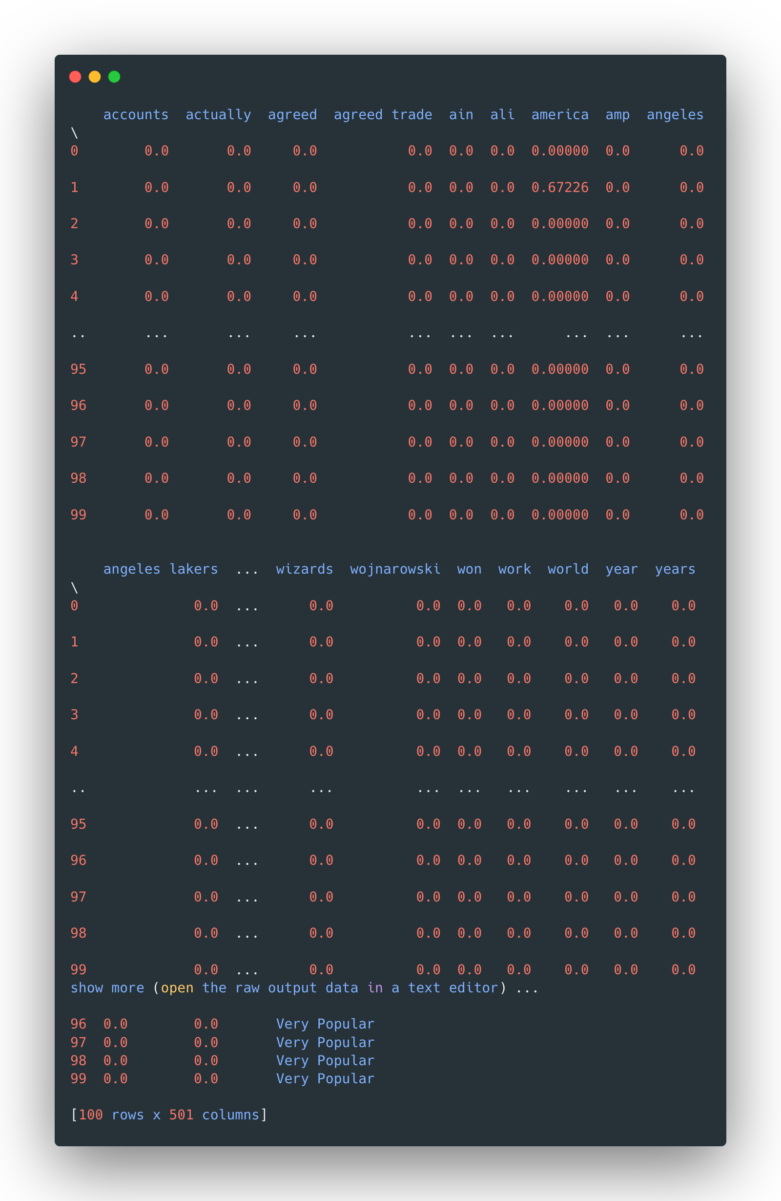
The tf-idf values are also standardized, although the matrix is still very sparse due to the nature of text data that not too many words are repeated in each document.

The general structure of the preprocessed data looks like this:

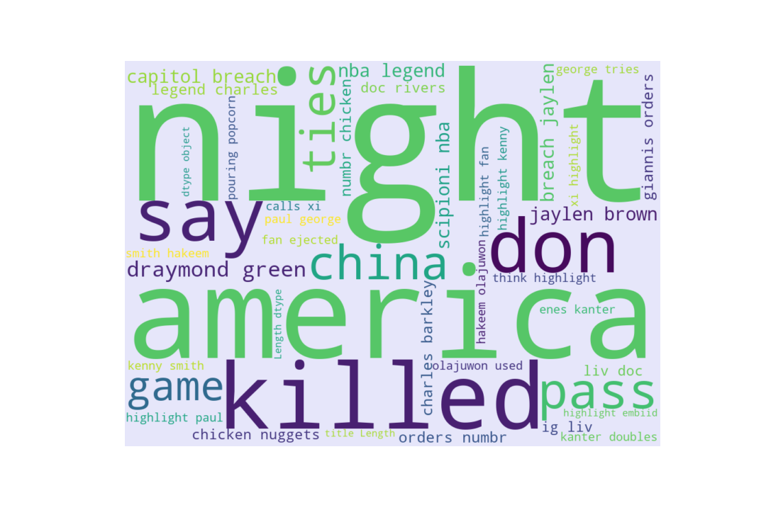
A wordcloud is also plotted like last time.

Of course, the text data is also split into a pair of 80-20 training/testing sets.

Model fitting

Then the preprocessed data is fitted in a multinomial naïve Bayes model. The resulted confusion matrix is plotted below:

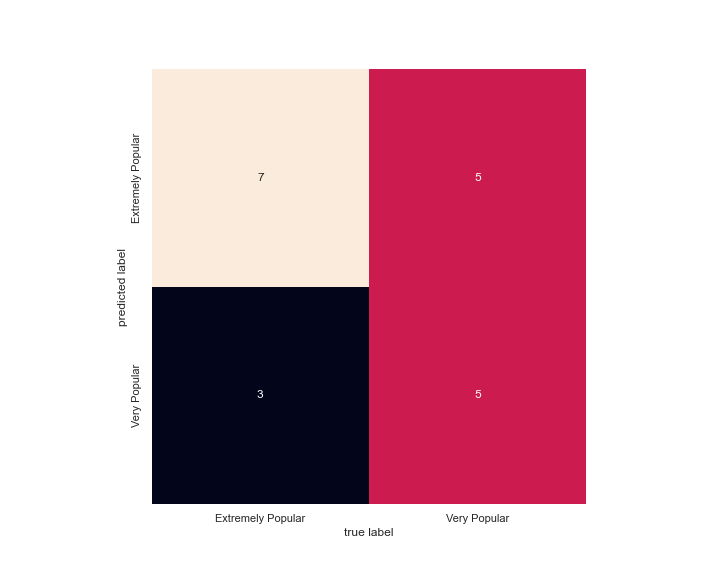
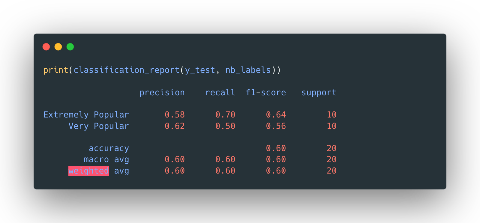
The overall accuracy is 60%.

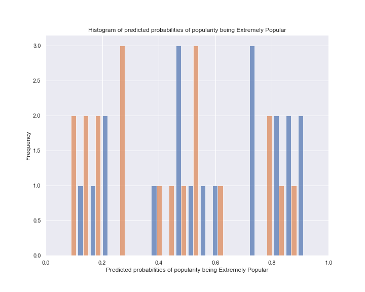
Furthermore, a naïve Bayes model in fact calculates the probabilties of each class. The following is a histogram displaying the probabilties of the test records to be both classes. Orange stands for Extremely Popular, while blue means Very Popular.

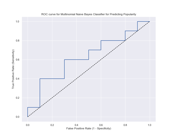
Finally, an ROC curve is plotted for the “goodness” of such a model, which will be discussed in the later paragraph.

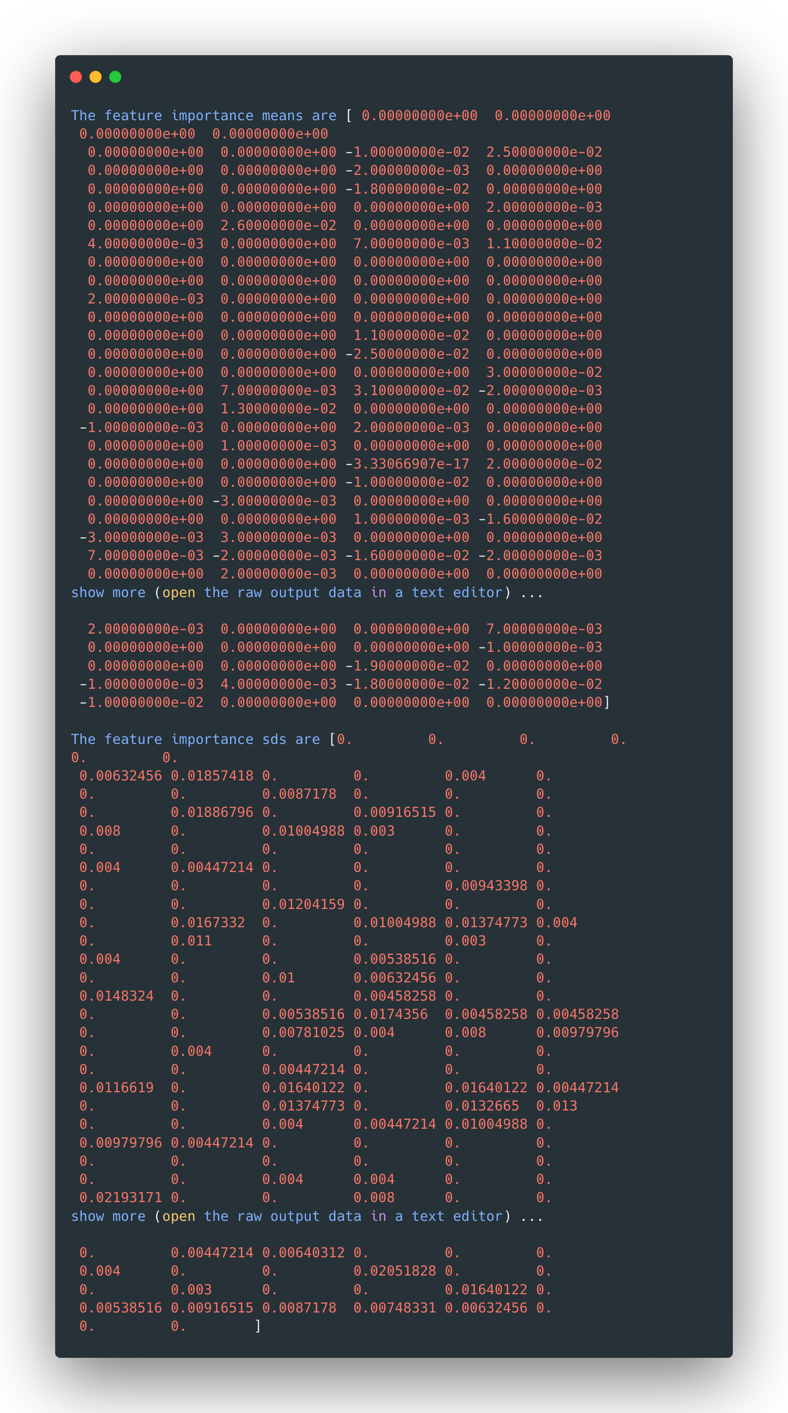
Feature importance

The feature importance of the naïve Bayes model on text data, can be represented in the following numpy array. Since the DTM of text data used in this part is rather large and sparse, the feature importance has a hard to interpret length of "relative importance" accordingly. A further dive into the data will reveal that the one with the most importance is the word "deep", which could be related to some amazing long-distance three-pointer shootings in the game.

Besides, the feature standard deviations are also included:

Interpretation

Without doubt, the naïve Bayes classifier with an accuracy of 60% is not ideal, especially for a testing data set of size 20. It’s just slightly better than flipping a coin, or randomly guess everything is of one class only. One could not even be sure if the 60% is just being “lucky”. It is almost conclusive to say that predicting the popularity barely based on the word choice of titles is impossible.

The ROC curve from the last plot also demonstrates the model's poor performance. In contrast, a decent model should close in the top left corner as much as possible.

Nevertheless, there are some highlights of such a model:

1. The training process is extremely fast. (Thanks to the small size of the data as well.)
2. The results are easy to interpret. A vector of probabilities will directly tell the reader what the model “thinks” the record belongs to.
3. The model almost does not need any tuning.

But we also need to be careful about the assumption that each variable should be independent of each other. This rarely happens in real life, including this case. Just imagine whether the occurrences of the following two words are independent:“Washington” and “Wizards”.

No models are perfect, some even fail its own assumptions.